Evaluation in designing a recommender system (Part 2)
This is the second article in the evaluation criteria series. You can find the introduction part here:
In this article, I focus on the prediction accuracy criterion, which is perhaps the most popular criterion for evaluating an RS in both academic and industrial fields.
I. Evaluation criteria
- Prediction accuracy
It’s a recommender system’s job to predict how much a user might like an item or how likely a customer will purchase a product. This prediction capability plays a vital role in the existence of an RS, and not surprisingly, this property is the most discussed in the field. Since this property is typically independent of the user interface and can thus, be measured in an offline experiment.
1.1 Rating Prediction Accuracy
Root Mean Squared Error (RMSE)
RMSE is perhaps the most popular metric used in evaluating the accuracy of predicted ratings. The system generates predicted rating uᵢ for a test set Ƭ of user-item pairs (u, i) for which the true rating rᵤᵢ are known. The RMSE between the predicted and actual ratings is given by:

This is a straightforward method to measure how far off predicted values are from ground truth ones. It’s intuitively easy to understand and one of the most widely adopted general-purpose evaluation metrics. Large errors have a disproportionately large effect on RMSE. Consequently, RMSE is sensitive to outliers.
Ƭ : test set of user-item pairs (u,i)
rui : true preference score
Mean Absolute Error (MAE)
MAE is a popular alternative to RMSE. Compared to MAE, RMSE penalizes large errors.

Normalized RMSE (NRMSE) and Normalized MAE (NMAE)
NRMSE and NMAE are versions of RMSE and MAE that have been normalized by the range of the ratings.

Average RMSE and Average MAE
If the test set has an unbalanced distribution of items, the average RMSE or average MAE might be better candidates. We can compute MAE or RMSE separately for each item or each user and then take the average overall items or users. By doing that, we relieve the heavy influence from a few very frequent items that happen to be in the dataset.
1.2 Usage Prediction
In many applications, a recommender system does not predict the user’s preferences of items, such as movie ratings, but tries to recommend to users items that they may purchase/use. Like the case of selling comics, we are interested not in whether the system properly predicts the ratings of these comics but rather whether the system properly predicts that a user will add these comics to his shopping list. In an offline setting, this type of prediction typically falls into one out of four cases.

In comic project context:
True Positive: An RS predicted a user will buy this comic, and it’s true.
True Negative: An RS predicted a user will NOT buy this comic, and it’s true.
False Positive: An RS predicted a user will buy this comic, and it’s false.
False Negative: An RS predicted a user will NOT buy this comic, and it’s false.
Then, we can count the number of predictions that fall into each cell in the table above and compute the following quantities:

Typically, we can expect a trade-off between these quantities — while allowing longer recommendation lists typically improves recall, it is also likely to reduce the precision.
1.3 Ranking Measures
In some applications, items can come in huge quantities. In such a scenario, it might be tempting to recommend only the best relevant items to users. Thus, a good ranking mechanism is tremendously important. There are two approaches for measuring the accuracy of a ranking: reference ranking and utility-based ranking.
1.3.1 Reference ranking
First, we construct a set of items in the correct order for each user (aka ground truth set), then measure how close a system comes to this correct order. Calculating the distance between the ground truth ranking list and the predicted one is a popular way to measure how well the RS ranks.
1.3.2 Utility-based ranking
Numerous research studies have shown users want the great recommendations to appear at the top of the list returned from an RS. That’s why taking recommendations’ positions into account when measuring the effectiveness of an RS is crucial. Here comes the definition of utility. The utility of each recommendation is the utility of the recommended item discounted by a factor that depends on its position in the list of recommendations. An RS is assumed to work well if it provides recommendation lists with a lot of not-so-discounted items.
Mean reciprocal rank (MRR) is a popular statistic measure for evaluating this type of ranking:

The premise of the metric is the more relevant item should be presented to a user before the less relevant one. This order appearance should reflect in the order of the recommendation list.
Where rankᵢ refers to the rank position of the first relevant recommendation for the i-th time the RS is used.
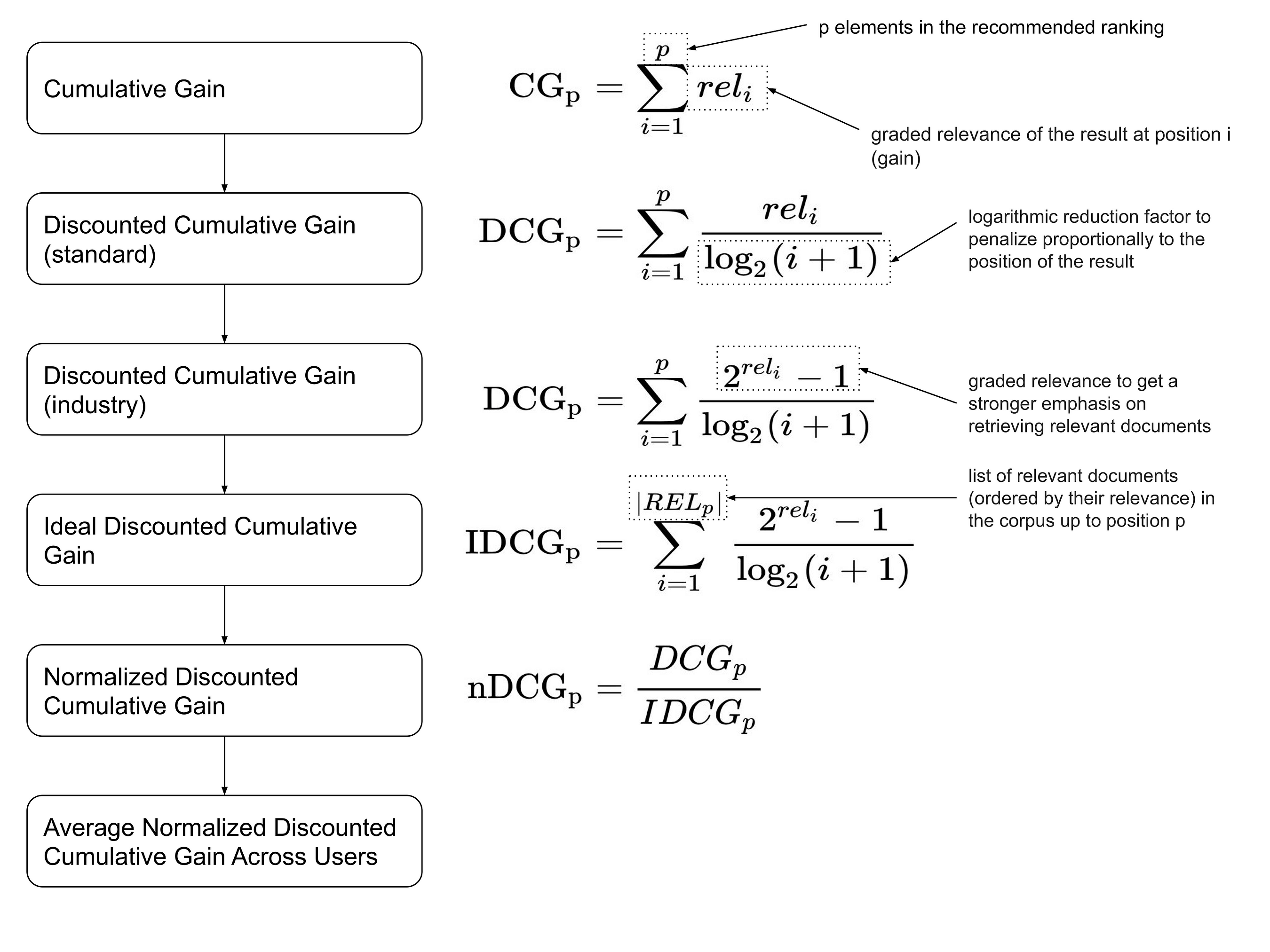
Normalized discounted cumulative gain (NDCG) is another alternative.

The formula mentioned above is just one popular way to calculate such a metric. However, depending on different situations, we might tweak it to produce desired effects. For example, the numerator part of DCGp can just be relᵢ put less importance on the ratings:

This metric measures the quality of ranking in a recommended list. In general, users prefer high relevant items to appear at top positions in the list. As the result, high NDCG values imply good ranking quality. As its formula suggests, the normalized DCG metric does not penalize irrelevant items in the recommended list. Also, NCDG may not be suitable for differentiating two recommenders that produce all relevant items. For instance, if considering an item with a relevance score > 3 relevant, then the NCDG scores for two lists [5,5,5] and [4,4,4] are the same.
Example: Let’s say we have a list of recommended items with relevance/preference scores as: L = [2,3,5,1,4]. With the aforementioned premise holds, the example list above should ideally be ordered as: Li = [5,4,3,2,1]

Another option is the Mean of Average Precision (MAP). With this metric, we compute the mean of average precision (AP) overall users. For an RS to have a high AP value, the recommendations not just have to be relevant, but they also have to be at the top of the recommended list.

Another option is the Mean of Average Precision (MAP). With this metric, we compute the mean of average precision (AP) over all users. For an RS to have a high AP value, the recommendations not just have to be relevant, but they also have to be at the top of the recommended list.

MAP is a harmonized metric between RMSE and NDCG since it includes both relevance and ranking in the formula. Thus, we consider this metric score a factor that reflects the overall performance of a recommender’s prediction capability.
Note: good balancing between precision and recall has always been an objective of any systems that need to return relevant results to end-users, including recommender systems. However, due to users’ experience concerns and the length of the recommended list is often fixed, precision is a more important factor in our case. Thus, MAP is a good metric in this case. However, according to its formula, the relevance of all items are treated equally ( always 1 if relevant), the metric score excludes the effect of relevance difference between items. Because of that reason, the metric needs to be used with other relevance prediction metrics to evaluate the system performance better.
Example: Let’s assume:
We have a 5-item recommended list: L = [A, B, C, D, F], N= 5. Based on some criteria, [B, D, F] is the relevant ones or the ones that have high preference scores, so m=3. The rest of the list is irrelevant. In other words, [A, C] should not be recommended to the users.

Note: I put all references used in my series in the last article.

Note: I put all references used in my series in the last article.
